LocoFlow
Please note this is an early release, there is little optimisation and it may have bugs I do not know about.
LocoFlow is tool for creating live and interactive diagrams that model systems. It is inspired by the diagrams found in Donnella H. Meadows’ book “Thinking in Systems,” LOOPY by Nicky Case and Machinations by Joris Dormans.
LocoFlow was designed and programmed by Luke Perkin.
The Nodes
Diagrams in LocoFlow consist of nodes and the connections between nodes. The main node in LocoFlow is called Stock which represents a stock of resources, such as money in a bank account, ore inside a mine or intangible resources such as happiness within a person.
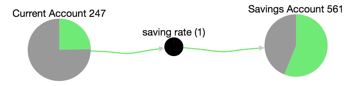
Resources move between Stocks via Valves. A Valve pulls resources from all its inputs and passes them along to all its outputs. The higher the valve’s flow value, the more resources it will pull. In fig 1 one unit will move from the current account to the savings account every tick.
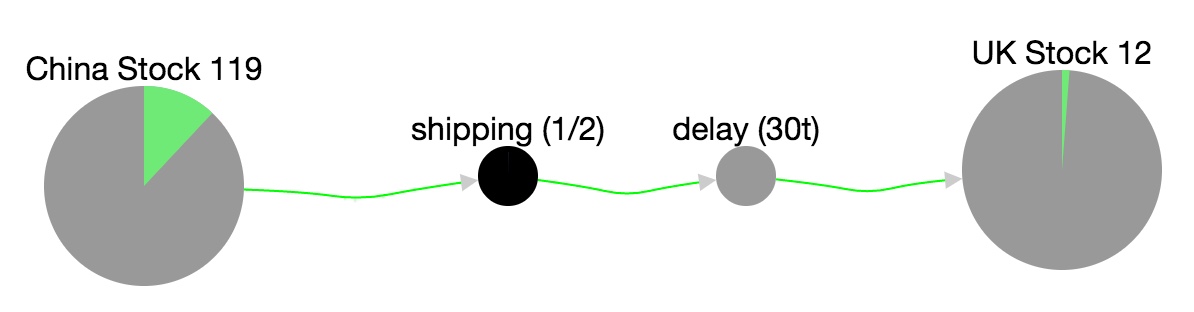
Resources take time to move along the connections, the further apart the nodes the longer it takes. This is useful for modelling latency found in many systems. If you want to exaggerate this latency you can use a Delay node. In fig 2 there will be a delay of 30 ticks to get stock from China to the UK.
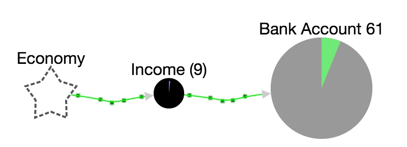
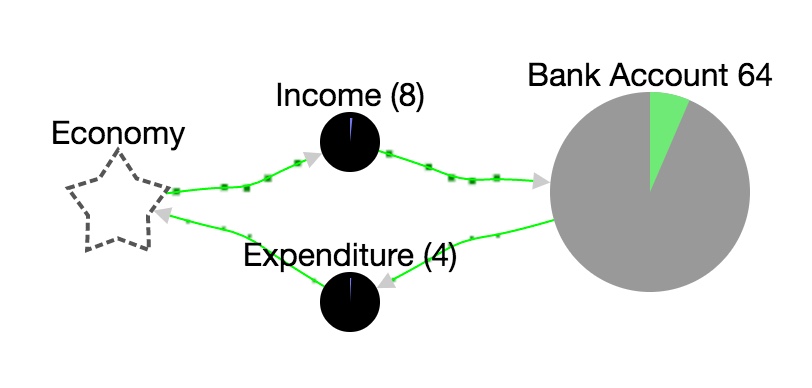
Stocks model finite pools of resources. If you wish to express an infinite source of resources, perhaps to indicate it’s coming from outside the system, you can use the External node. In fig 3 the star represents the external source. In fig 3.1 you can see that resources can go into external nodes, which will destroy those resources.
External nodes also have an advanced feature for generating resources based on an expression, read more about that here.
Connections
There are three types of connections in LocoFlow. You’ve already seen one of them which is called a resource connection, they’re the green arrows. There are also state connections and condition connections.
State Connections
These represent the flow of information. If a stock’s quantity goes from 10 to 20 it will send a +10 signal along all the outgoing state connections. If the same stock were to drop back to 10 it would send a -10 signal. Like resources, these signals take time to travel. Using state connections allow you to model feedback systems. For example in fig 4 there is a state connection going out of the bank account and in to the valve. Whenever that bank balance increases it sends a signal to the valve to increase its flow rate, which in turn increases the bank balance. This is called a positive feedback loop.
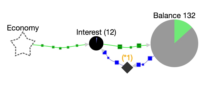
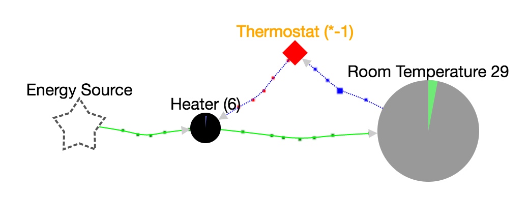
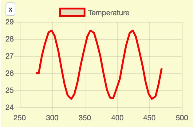
The diamond shape you see in fig 4 is called a multiplier. In this case it’s just used to keep the diagram tidy but you can change its multiplier to change the effectiveness of the feedback loop, or even make it a negative multiplier. In fig 4.1 as the heater warms the room the stock sends a positive signal, but the multiplier inverts this signal causing the heater to reduce its flow rate. The room temperature will start to stabilise.
You can also link a state connection direct to a stock node, in which case it will act like a resource. The key difference between a resource and state is that when resources reach a junction, such as a valve with multiple outputs, they distribute evenly. A state signal is always copied to all outputs.
Condition Connection
The pink connections are only meant to be used with the condition nodes. When connected to a stock or a valve the condition node will check each tick if the condition is true. For example you may want to check if a stock is over a certain amount.
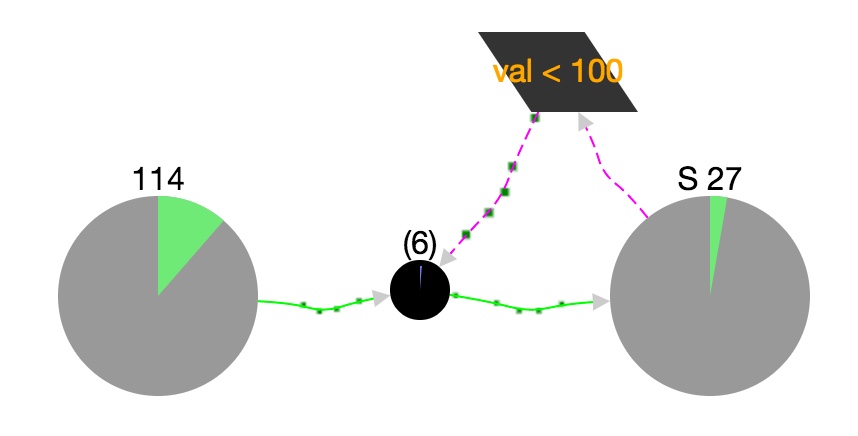
The condition is a single expression (in javascript) that evaluates to a truthy value. When the expression evaluates to false it will output a disable signal, which will shut off all the valves it’s connected to. The val variable is the current quantity in a stock and the flow variable is the valve’s flow rate.
Generator
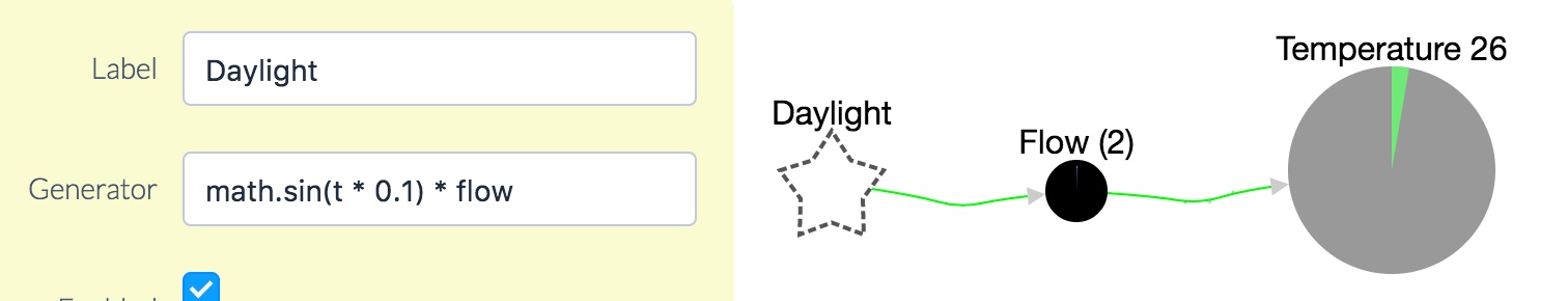
External nodes have an extra field called generator. This is a javascript expression that must evaluate to a number. This can be used to model external sources with varying output. Fig 6 shows how you can use generators to model daylight.
Tools used.
- Cytoscope.js
- Vue.js
- Chart.js
- ElementUI
- Mousetrap